Methodology.
i.e. How was the data collected and wrangled?
Site

Zoological Museum, Copenhagen Denmark (image link)
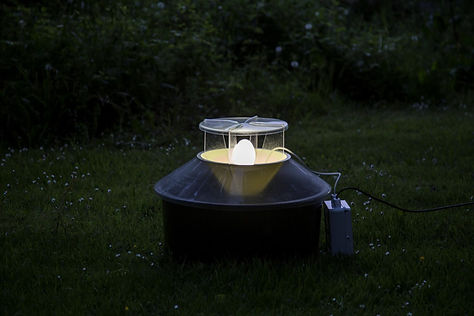
Robinson light trap, may not be exact trap used in study (image link)
The study site was the rooftop of the Zoological Museum at the University of Copenhagen (Denmark), where insect counts from a Robinson light trap were recorded between 1992-2009 (Thomsen et al., 2016). The singular modified light trap was 17.5 m above the ground and was equipped with a 250W mercury vapor bulb as a light attractant and 1,1,2,2-tetrachlorethane as a killing agent (Thomsen et al., 2016). Because insects can disperse quite easily, it was assumed that the recordings at the site were representative of the general communities of insects within the city of Copenhagen.
Copenhagen is Denmark's largest city and capital. It lies on the coast, facing the strait that separates Denmark from Sweden. Precipitation usually ranges from 45-82 mm, with April being the dryest month and August being the wettest (climate-data.org). Average temperatures usually range from 0-18 degrees Celsius, with January being the coldest month and July being the hottest (climate-data.org).
Explore the study site using the map below!
Data Decisions.
Individual insects from the Orders Lepidoptera and Coleoptera were originally counted and classified to the species level every 10 days from the singular light trap (Thomsen et al., 2016). However, for the purposes of this project, and to reduce overcomplexity, insects were analyzed only at the Family level and total monthly insect counts were used. In addition, only Families who had at least one total monthly count greater than or equal to 50 individuals were included in the analyses. By narrowing the scope of Families that were analyzed, it was hoped that general trends about the common insect communities in Copenhagen would be made instead of focusing on rare groups within the communities. Finally, traps are known to only have run consistently from April to November (Thomsen et al., 2016) and so all other months' data were removed from the dataset. Finally;
Three major assumptions about the insect data were made;
1.
that light traps ran every day of the year between the months of April and November, for all years with data
2.
that missing data for any given Family indicated a count of zero for that time frame
3.
that there was no insect avoidance of the traps due to take-down and set-up of the traps
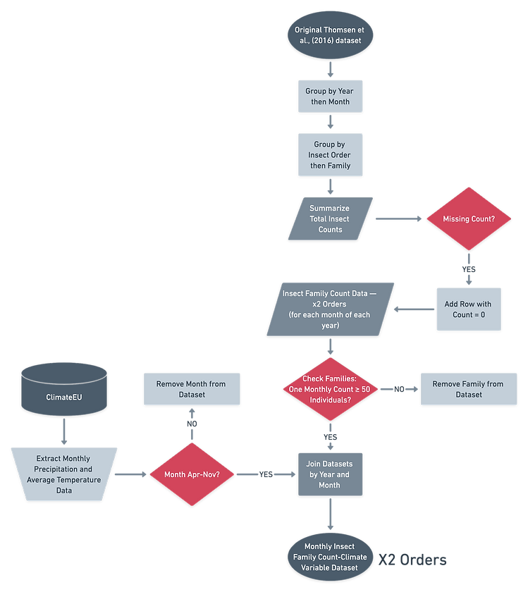
It is important to note that these assumptions differed from those made in other works using this dataset (Thomsen et al., 2016). Figure 4 shows the data cleaning methods applied to the original datasets.
Figure 4: Flow chart of the data cleaning methods performed on Thomsen et al.'s (2016) insect count dataset and Climate EU's precipitation and temperature records (Marchi et al., 2020) for Copenhagen, Denmark between 1992-2009.
.png)
Statistical Analyses.
The statistical analyses for this project can be broken down into 3 strategic steps. The first step aims to visually assess the temporal trends of insect abundance. The second step aims to visually assess the relationships between deviations in climate variables from average values and insect abundance. Finally, the third step aims to quantify the relationships between climate variables and insect abundance within distinct temporal time frames. The following statistical analyses were performed for each of these steps;
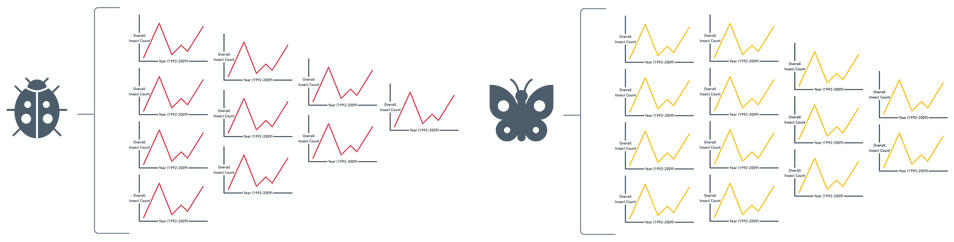
Step 1.
Yearly insect counts were plotted for each year of the data. A separate plot was created for each Family. This way, boom-bust patterns could be identified. These types of trends are important to understand in order to properly interpret other results.
Step 2.
Monthly insect counts were plotted against their respective climate variable deviations from average monthly values. Temperature deviations were calculated as the difference between the observed value and the average value for the respective month. Precipitation deviations were calculated as the percent equivalent of the observed values compared to the average value for the respective month. This permitted exploration of the possible insect responses to extreme weather events among the insect community.
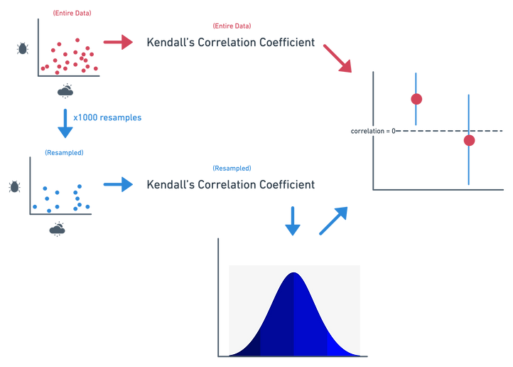
Step 3.
Kendall correlation coefficients (tau) were calculated between monthly deviations in climate variables and monthly insect counts of each Order. P-values were adjusted for the 8 statistical tests run using the holmes method of adjustment; this was done simply to compare with the bootstrapped significance determinations. Adjusted p-values less than 0.05 were considered significant. 95% confidence intervals were calculated for each correlation coefficient using bootstrapping methods (B = 1000). Coefficients with confidence intervals that were fully above or below the value of 0 were considered significant. This type of analysis was chosen to accurately determine which months and their respective climate variables influenced the observed insect abundances the most.
.png)
A Kendall correlation coefficient was used because the data did not meet the assumption of normality of other parametric correlation methods. The assumptions of the Kendall correlation test are that the data;
-
are ordinal or continuous
-
have a monotonic relationship
The insect-climate variable data met both of these assumptions and the bootstrapped confidence intervals answered this project's research question quite effectively. Bootstrapped methods do not need to assume normality due to the Central Limit Theorem. Other non-parametric correlation alternatives include the Spearman correlation coefficient. The Kendall correlation coefficient was chosen instead because it is more robust to outliers.